Full End-to-End Machine Learning API


![]()


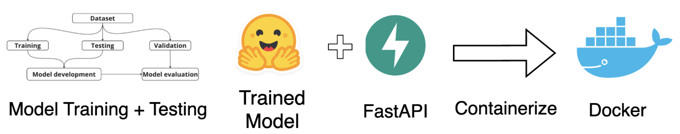
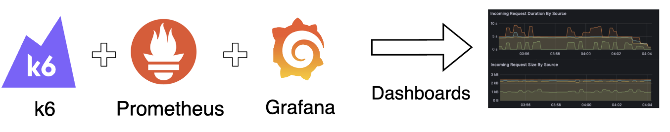
In this project, I deploy a Hugging Face DistilBERT sentiment model behind a FastAPI service, containerize it with Docker, run it on Kubernetes using AWS EKS, add Redis caching, and validate behavior under load with k6 + Grafana.
You can check out the code to this project here.
Prototype vs Production
Prototypes are optimized for speed. With Hugging Face, you can load a pretrained model and run inference quickly. However, in production, the problem shift from "does it work?" to "does it keep working?"
The first hurdle is reproducibility. Code that runs on your machine can break on another machine due to dependency issues. Docker fixes this by packaging the API + model into a single artifact such that the service behaves the same everywhere. After that comes reliability. Even a perfect container still needs an operator, something to restart failures, route traffic, and scale when usage spikes. Kubernetes provides that runtime layer, while FastAPI gives clients a stable interface through prediction endpoints.
Performance is usually the next pain point. If inputs repeat, re-running inference is wasted work. Redis adds a cache so repeated requests can return quickly and reduce compute load. To simulate real-world behavior, k6 is used to apply controlled load, and Grafana visualizes latency and throughput so performance shifts show up in metrics instead of surprises.
Model + API
The model used in this project is a Hugging Face DistilBERT sentiment classifier,
I fine-tuned the model and exported everything which includes the model weights (
model.safetensors, pytorch_model.bin) and the tokenizer/config artifacts
(config.json, tokenizer.json, vocab.txt). Altogether, the bundle is roughly
1GB, which is why packaging and deployment choices matter (more on this later).
I wrapped the model in a FastAPI service that exposes two main endpoints:
/project/health- used for Kubernetes readiness + liveness checks/project/bulk-predict- performs batched sentiment prediction
The API accepts an array of text strings and returns a JSON response with ranked sentiment labels and confidence scores, designed to be easy to plug into downstream systems.
curl http://localhost:8000/project/health

{"status":"healthy"}
curl -X POST "http://localhost:8000/project/bulk-predict" -H "Content-Type: application/json" \
-d '{"text":["i love this","this is bad"]}'
{
"predictions": [
[
{"label": "POSITIVE", "score": 0.99},
{"label": "NEGATIVE", "score": 0.01}
],
[
{"label": "NEGATIVE", "score": 0.98},
{"label": "POSITIVE", "score": 0.02}
]
]
}Dockerizing the API + Model
A Dockerfile is the blueprint for building a container image: it defines the base runtime, what files get copied in, and the commands needed to install dependencies and start the API. The main design choice is single-stage vs multi-stage. A single-stage build is simpler because everything happens in one image, but it often ships extra build tools. A multi-stage build separates "build/install" from "runtime": the builder stage installs heavy dependencies and creates the environment, then the final stage copies in only what's needed to run the service usually producing a leaner runtime image.
Infrastructure Configuration

After containerizing the service, I deployed it on Kubernetes using
AWS EKS so the API can run reliably outside a single machine.
The cluster is configured with a public endpoint in us-east-2 running Kubernetes 1.34.
Workloads run on a small node group (t3.medium, 1 node, AmazonLinux2023, 20Gi root volume).
Conceptually, Kubernetes makes this project always on runtime. Instead of running a single server process,
I describe the desired state (pods, services, scaling rules) in YAML and let the control plane keep reality aligned.
If a container crashes, Kubernetes recreates it. If the node goes away, Kubernetes reschedules pods onto a healthy node.
And because clients talk to a stable Service name instead of a changing pod IP, traffic keeps flowing even
as pods restart or get replaced.
Redis is deployed alongside the API as an in-cluster dependency. The API uses REDIS_URL pointing at the Redis Service DNS name,
so the application never needs to know pod IPs. When requests repeat, Redis enables fast cache hits and avoids
rerunning model inference, reducing latency and lowering CPU pressure.
Base Manifests
In base/, the two key objects are Deployment and Service.
A Deployment is Kubernetes replication controller, it declares how many pod replicas should exist and what container image + settings they run.
If a pod exits (crash, OOM, node drain), the Deployment ensures a replacement pod is created so the system converges back to the desired replica count.
A Service provides a stable DNS name (and virtual IP) in front of those pods. That's why the API can reference Redis as
redis-service:6379, it's service discovery by name, not by fragile pod IPs.
The API Deployment also uses three health probes on /project/health. Startup gates the initial boot so slow model load
doesn't get treated as a failure. Readiness controls whether a pod receives traffic (only "ready" pods get added behind the Service).
Liveness catches deadlocks or bad states and triggers a restart. Together, these probes make the service resilient to the most common
production failure modes such as slow cold starts, partial initialization, and unhealthy but running processes.
Production Overlay (overlays/prod/)
The production overlay uses Kustomize to apply environment specific changes on top of the same base.
The namespace isolates prod resources, and the images section swaps project:latest
into the pinned ECR image tag, which is how the cluster runs the exact build pushed.
The HPA adds elasticity during spikes, Kubernetes can increase the number of API pods up to the configured maximum, then scale back down when traffic drops.
Finally, the VirtualService defines external routing rules so requests get routed to the API Service, while Kubernetes continues
to load balance across healthy pods behind the scenes.
Load Testing (k6)
Once the API is deployed, the next question becomes: how does it behave under real traffic? In production, requests rarely arrive at a perfectly steady rate. Instead, systems see ramp-ups, steady plateaus (normal usage), and ramp-downs (traffic fades). They also see a mix of repeated inputs (cache hits) and novel inputs (cache misses) which is especially important for inference workloads where "misses" tend to be CPU-heavy.
To simulate that behavior, I used k6 to generate controlled HTTP traffic against the
in-cluster service DNS. Running the load generator inside Kubernetes isolates the measurement to application + cluster behavior
(rather than public internet variability). The test ramps from 0 to 10 virtual users, holds steady, then ramps back to 0.
Each user repeatedly calls /project/bulk-predict with a payload that has a configurable cache rate—so we measure performance under a realistic
mix of cache hits and cache misses.
During the run, I track two layers of metrics. First, request-level performance: latency percentiles (especially p95/p99), throughput (requests/sec), and error rate (non-2xx responses). Second, system behavior: pod CPU pressure (what drives HPA decisions), replica count changes, and how quickly the service recovers from load spikes. These metrics tell whether the service remains responsive, whether scaling kicks in when needed, and whether caching actually reduces compute load under repeat traffic.
Load Simulation (k6)
The test is packaged as a Kubernetes Job so it runs the same way every time with a known k6 version, a fixed script, and a clean lifecycle. The output gives immediate feedback (latency distributions and pass/fail thresholds), while the cluster-level monitoring shows whether latency increases are tied to CPU saturation, scaling delays, or cache miss pressure.
Run output (simulate.js)
(10m29.0s), 01/10 VUs, 2866 complete and 0 interrupted iterations default [ 100% ]
01/10 VUs
10m29. 0s/10m30. 0s
running (10m30.0s), 01/10 VUs, 2869 complete and 0 interrupted iterations default [ 100% ]
01/10 VUs 10m30.0s/10m30.0s

THRESHOLDS
http_req_duration
✗ 'p(99)<2000' p(99)=5.07s

TOTAL RESULTS
checks_total: 2870
checks_succeeded: 100.00%
checks_failed: 0.00%

HTTP
http_req_duration: avg=1.86s min=2.15ms med=58.5ms max=5.56s p(90)=4.58s p(95)=4.75s p(99)=5.07s
http_req_failed: 0.00%
http_reqs: 2870 (4.555271/s)

EXECUTION
iteration_duration: avg=1.86s min=2.28ms med=68.21ms max=5.56s p(90)=4.58s p(95)=4.75s
vus: 1 (min=1 max=10)
vus_max: 10 (min=10 max=10)

NETWORK
data_received: 2.3 MB (3.7 kB/s)
data_sent: 1.1 MB (1.7 kB/s)
How to interpret this run
- Reliability is good: 0% failed requests and 100% checks passing means the API stayed up and returned HTTP 200s.
- Median is fast, tail is slow: a ~58ms median alongside a ~5s p99 indicates some requests return quickly (cache hits), but a smaller fraction take several seconds (cache misses).
-
The SLO failed: the enforced threshold was
p(99)<2s, but the observed p99 was ~5.07s. This is exactly where monitoring helps: Grafana makes it obvious that tail latency rises even when throughput and success rate look healthy.
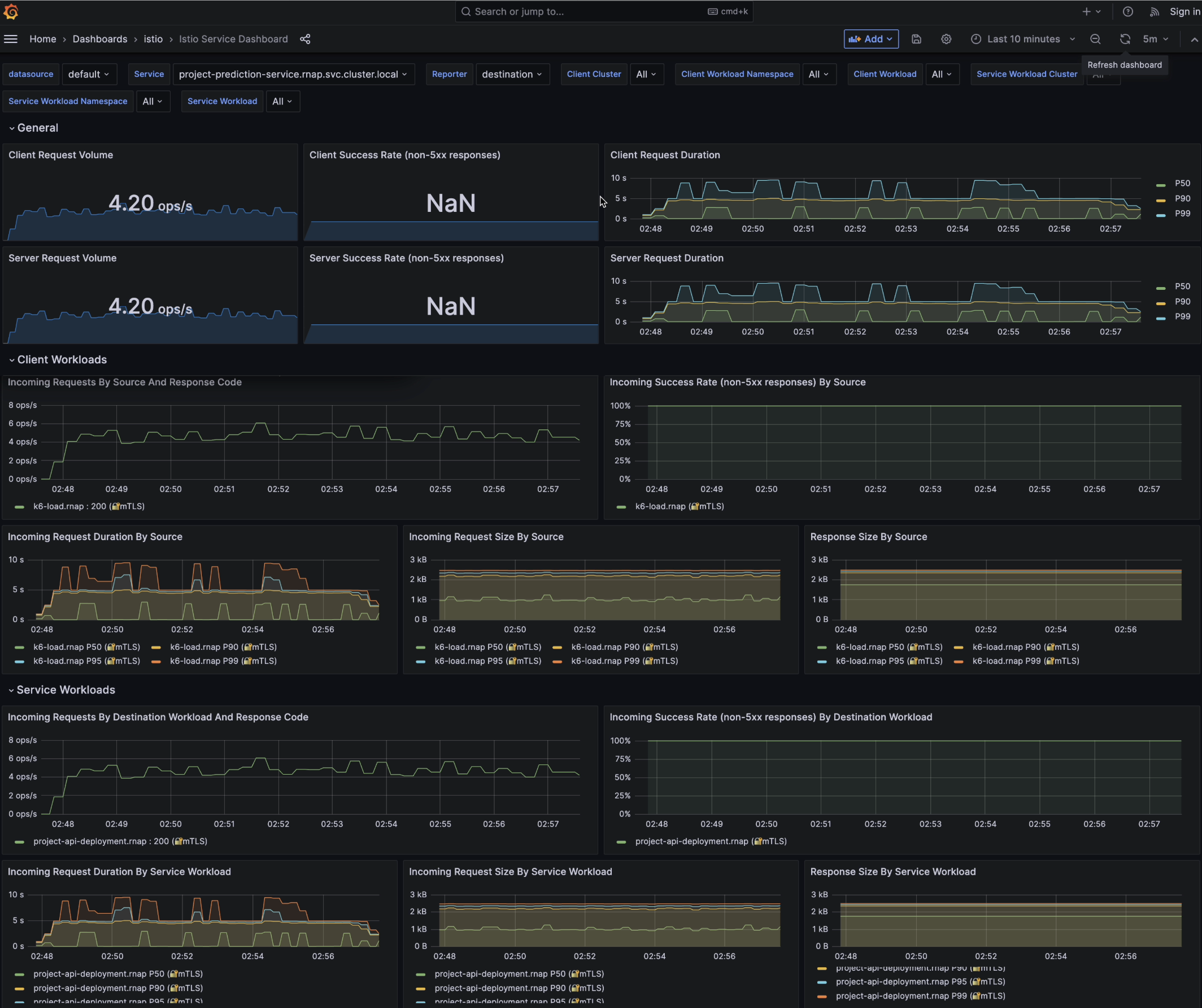
Monitoring (Grafana)
With the API deployed and k6 generating load, the last piece is understanding how the system actually behaves. Istio sidecars emit rich telemetry to Prometheus, and Grafana turns that data into dashboards. This section showcases how our system performs under load and answers: what does Redis caching do to end-to-end latency under steady traffic?
To answer that, I ran the same k6 workload twice:
- Cache disabled -
CACHE_HIT_RATE = 0.0 - Cache always used -
CACHE_HIT_RATE = 1.0
The request rate, payload size, cluster configuration, and test duration are identical between runs. That means any difference in latency is due to whether responses are computed fresh or served from Redis.
1. Verifying Load and Experiment Validity
First, I use the Incoming Requests By Destination Workload And Response Code panel to verify the basic shape of the experiment.
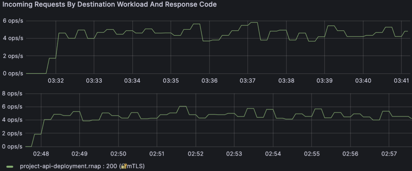
Incoming requests to project-api-deployment.rnap with Redis cache
disabled (top) and enabled (bottom). Throughput stays around 4-6 ops/s with
consistent HTTP 200s in both cases.
Both runs show:
- Steady throughput around 4-6 ops/s
- All responses as HTTP 200
- No spikes of 4xx/5xx errors
This tells us the workload is stable and the service is healthy. If latency changes, it's not because the traffic pattern collapsed or the app started throwing errors, rather it's because caching changed the work being done per request.
2. Latency Distribution by Percentile
The most important panel for this project is
Incoming Request Duration By Service Workload, which shows
the latency percentiles seen by
Istio for traffic hitting the
project-api-deployment.rnap workload.
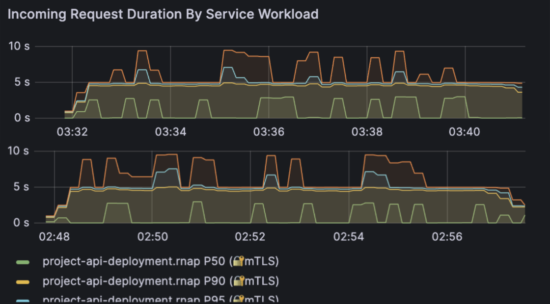
P50 / P90 / P95 / P99 request duration for the API with cache disabled (top) versus cache enabled (bottom).
The panel plots four key percentiles:
- P50 - median latency (the "typical" request)
- P90 - upper-end latency under load
- P95 - late tail where users start noticing slowness
- P99 - the slowest 1% of requests (hard tail)
The percentile definition is: Pk = latency value where k% of requests are faster and (100 - k)% are slower.
Tail latency (P95/P99) is what users feel when the system is stressed. You can have a median of 5s and still deliver a bad experience if 1-5% of requests take several seconds.
2.1 Cache Disabled (CACHE_HIT_RATE = 0.0)
With the cache disabled, every request runs full DistilBERT inference: tokenize, batch, compute logits, and post-process. In the Grafana panel, this shows up roughly as:
- P50 hovering around 4-5 seconds
- P90 closer to 6-8 seconds
- P95 flirting with the upper single digits
- P99 occasionally spiking into the 8-10 second range
The curves are also fairly "jagged", which means the latency distribution moves around as the node's CPU and memory pressure change. This is what we expect when every request is CPU-bound and there is no caching to smooth out work.
2.2 Cache Enabled (CACHE_HIT_RATE = 1.0)
In the second run, every request is a cache hit. The code path becomes:
cache miss path: Tnocache = Ttokenize + Tinference + Tpostprocess
cache hit path: Tcache ≈ Tredis_lookup + Tnetwork
Redis lookups are dramatically cheaper than running a transformer model, so the panel now shows:
- Lower P50 (median latency)
- Compressed P90, P95, and P99
- Much smoother curves with fewer spikes
In other words, caching makes the average request faster and also makes the worst requests less bad which is exactly what we want in a production system.
2.3 Quantifying the Improvement
To reason about the benefit, it's helpful to look at relative reduction:
L₀(Pk) = latency at percentile k with cache disabled
L₁(Pk) = latency at percentile k with cache enabled
Pk = (L₀(Pk) - L₁(Pk)) / L₀(Pk) × 100%
In my runs, the reductions roughly fell into the following ranges:
- P50: around 5-15% lower
- P90: around 10-20% lower
- P95: around 10-20% lower
- P99: around 15-25% lower
The higher the percentile, the more caching helps. That's a strong signal that Redis is eating the heavy tail of repeated requests and preventing them from turning into multi-second outliers.
3. Workload Consistency: Request Size
The Incoming Request Size By Service Workload panel is a sanity check that the experiment stayed fair.
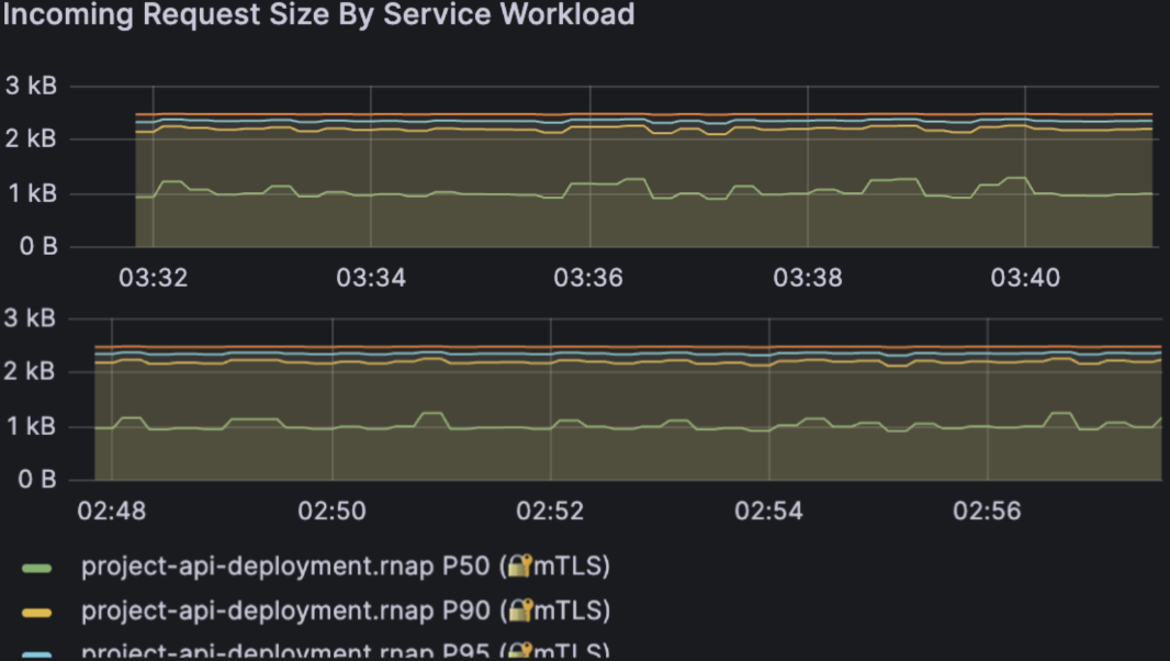
Request payload sizes remain stable between runs, so performance differences come from caching, not from different input sizes. In both runs, payload size sits around the same 1-2.5 kB band. That means:
- I didn't accidentally send smaller requests in the "faster" run.
- Network overhead stayed essentially constant between configurations.
Combined with the earlier throughput panel, this confirms that we're comparing apples to apples: same request rate, same request size, same cluster, only the cache behavior changed.
4. Omitted Panels
The full Grafana dashboard also includes several other panels such as Incoming Requests By Source And Response Code, Incoming Request Duration By Source, Incoming Request Size By Source, and Response Size By Service/Source.
I intentionally left these out for two reasons:
-
They duplicate the same story. In this experiment there is
only one logical client (
k6-load.rnap) and one backend workload. The "by source" panels have almost identical shapes to the "by service workload" panels, so including both would not bring new insight. - Response size is nearly constant. The sentiment API always returns the same small JSON structure for each input text. The response-size panels are almost flat lines; they're useful for sanity-checking that nothing weird is happening, but they don't help explain meaningful changes.
For a real multi-service mesh with many callers, the "by source" views would be critical to identify noisy neighbors or misbehaving clients. In this controlled, single-client benchmark, they're redundant - so I focus on the three panels that directly support the caching story: request volume, request duration, and request size.
5. Key Takeaways
Putting it all together:
- Reliability stays high. Even under continuous traffic, the service returns 100% HTTP 200s in both cache and no-cache runs.
-
Throughput is stable. The API comfortably sustains ~4-6
req/s on a single
t3.mediumnode with a 1-replica Deployment. - Tail latency is where caching shines. Median latency improves, but the biggest gain is in P95 / P99.
- Workload fairness is preserved. Request size and traffic shape are controlled, so we can directly attribute the improvement to Redis.
If this service were running in production, enabling Redis with a realistic cache key strategy would:
- Lower perceived latency for repeat traffic
- Reduce CPU burn on the node (fewer full model inferences)
- Give the HorizontalPodAutoscaler more headroom before scaling out
- Improve resilience during short traffic spikes
In that sense, caching is an architectural lever that improves user experience, resource efficiency, and system robustness at the same time. The Grafana dashboards make all of this visible in a way that's hard to argue with which is exactly what we want when running ML workloads on real infrastructure.
Closing Thoughts
This project started as “serve a model behind an API”, and ended up looking much more like a real production system: containerization for reproducibility, Kubernetes for resilience, Redis for performance, and load testing + dashboards to validate behavior with evidence instead of guesswork.
What I observed
- Reliability stayed strong under load: k6 reported 0% failed requests and 100% checks passing, and Grafana confirmed steady HTTP 200 responses.
- Throughput was stable: the system sustained about ~4-6 requests/sec during the steady state portion of the run.
-
Tail latency was the main bottleneck:
the median stayed low (cache hits), but P95 /
P99 rose into the multi-second range (cache misses / CPU-bound),
causing the
p(99)<2sSLO threshold to fail. - Caching helped most where it matters: enabling Redis compressed the tail P95 / P99 and made the latency curve smoother, reducing bad experiences even when average behavior looks fine.
What I would improve next
- Reduce cold-start and per-request compute: explore a smaller model, optimized inference runtime, and batching controls to reduce CPU pressure.
- Improve cache strategy: use a more realistic cache key (normalized text), measure hit-rate explicitly, and add TTL + eviction tuning so Redis remains useful as traffic changes.
- Scale on the right signal: HPA on CPU works, but inference services often benefit from scaling on request rate / queue depth or custom metrics. Kubernetes makes this easy to evolve over time.
-
Make SLOs actionable:
keep the
p99threshold, but add alerting that ties spikes to root causes (CPU saturation, replica count changes, cache miss spikes) using Prometheus + Grafana.
Final thoughts
The core lesson is that production ML is less about "running a model" and more about building a system that is repeatable, observable, and robust under real traffic. Docker + Kubernetes make deployment predictable, Redis shifts work away from expensive inference, and k6 + Grafana turn performance into something you can measure, debug, and improve iteratively.
If you're building something similar, the fastest way to level up is to treat your model like any other production dependency: define health checks, enforce SLOs, test under load, and let metrics drive the next optimization.
If you'd like to discuss ML systems, distributed inference, or production deployment feel free to reach out 😊